1 Introduction

As I’ve said in one of my previous posts, Rob J. Hyndman has excellent book on forecasting that is full of exercises by the end of each chapter. One of those chapters - to be more precise, Chapter 8 - Exponential Smoothing - has tasks that require the implementation of ETS. This really helped me to understand ETS. But, before I go into that part, let’s see what theory says about ETS.

2 Theory

Hyndman says the following on ETS:

Exponential smoothing was proposed in the late 1950s (Brown, 1959; Holt, 1957; Winters, 1960), and has motivated some of the most successful forecasting methods. Forecasts produced using exponential smoothing methods are weighted averages of past observations, with the weights decaying exponentially as the observations get older. In other words, the more recent the observation the higher the associated weight. This framework generates reliable forecasts quickly and for a wide range of time series, which is a great advantage and of major importance to applications in industry.

He also goes on to say that ETS (to be more precise, SES or simple exponential smoothing) is most suitable for forecasting data with no clear trend or seasonal pattern. The math behind the ETS is presented in 2 ways: through weighted average form and through component form. From the programming standpoint, I like component form better, but let’s present both approaches.

2.1 Weighted form

$\begin{matrix} (1) & {\hat{y}}_{T + 1 | T} = α y_{T} + (1 - α) {\hat{y}}_{T | T - 1} \end{matrix}$

Meaning of these mathematical symbols is as follows:

${\hat{y}}_{T + 1 | T}$ : first (forecasted) future value ( $T + 1$ ), given last historical value ( $T$ ).
${\hat{y}}_{T}$ : last historical value.
${\hat{y}}_{T | T - 1}$ : last forecasted value at index $T$ . Spoiler alert: this is where magic happens.
$α$ : smoothing parameter.

${\hat{y}}_{T | T - 1}$ is where the magic happens. Fitted values in ETS are one-step forecasts of the training data, and by deduction we can conclude that:

$\begin{matrix} (2) & {\hat{y}}_{T + 1 | T} = \sum_{j = 0}^{T - 1} α (1 - α)^{j} y_{T - j} + (1 - α)^{T} l_{0} \end{matrix}$

Hold your horses, you’re probably having questions about $l_{0}$ . We will get to that term in a minute, but when you see this term, read it as starting value.

2.2 Component form

The component form will get us to the same results, but it’s actually easier to see what is really going on. It consists of one simple equation, which we (surprise, surprise) call the forecast equation:

$\begin{matrix} (3) & {\hat{y}}_{t + h | t} = l_{t} \end{matrix}$ Same as before: future value, given the historical value ( ${\hat{y}}_{t + h | t}$ ) is equal to $l_{t}$ . But what is that? That we call the smoothing equation, and it’s given by the following formula:

$\begin{matrix} (4) & l_{t} = α y_{t} + (1 - α) l_{t - 1} \end{matrix}$

This is identical to the first formula in the weighted form, only the symbols are different. That’s it.

Okay, enough with the theory. Let’s implement this.

3 Implementation

Exercise 1 is as follows:

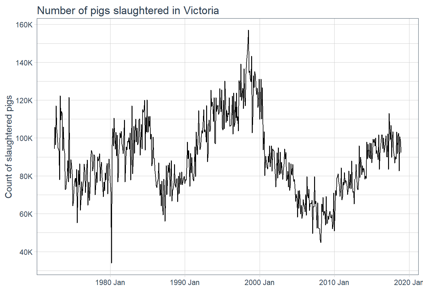
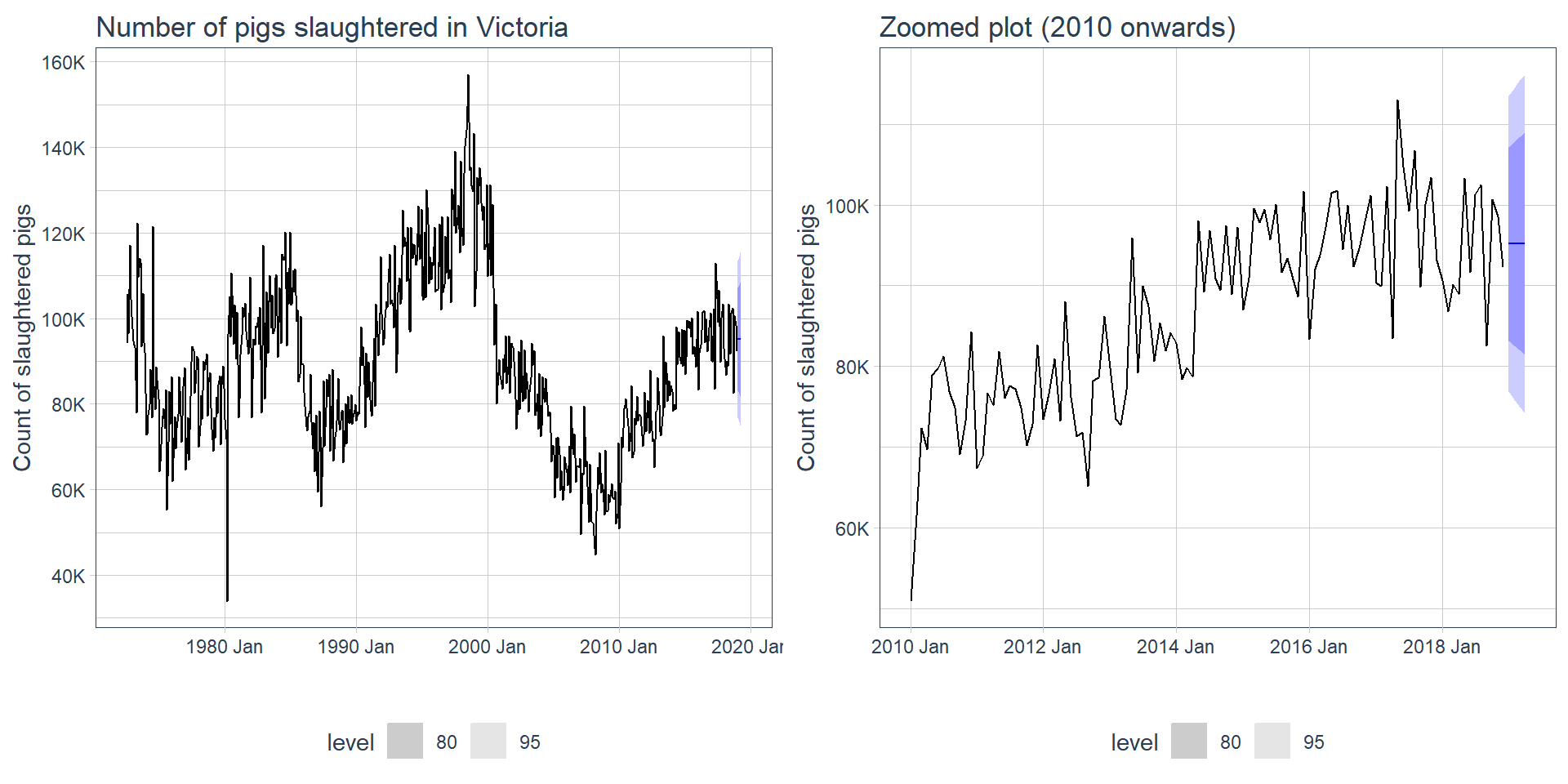
Consider the the number of pigs slaughtered in Victoria, available in the aus_livestock dataset. Use the ETS() function to estimate the equivalent model for simple exponential smoothing. Find the optimal values of $α$ and $l_{0}$ , and generate forecasts for the next four months.

tidyverse and fpp3 is loaded, so we can go on with the solution.

aus_pigs <- aus_livestock %>% 
    filter(str_detect(Animal, "Pigs") & str_detect(State, "Victoria")) %>% 
    select(Month, Count)

autoplot(aus_pigs, .vars = Count) +
    scale_y_continuous(labels = scales::label_comma(1, scale = 1/1e3, suffix = "K"),
                       breaks = seq(0, 200e3, 20000)) +
    labs(y = "Count of slaughtered pigs", x = "",
         title = "Number of pigs slaughtered in Victoria")

Let’s forecast with ETS using tools from fable:

fit <- aus_pigs %>% 
    model(ETS(Count ~ error("A") + trend("N") + season("N")))

report(fit)

Series: Count 
Model: ETS(A,N,N) 
  Smoothing parameters:
    alpha = 0.3221247 

  Initial states:
     l[0]
 100646.6

  sigma^2:  87480760

     AIC     AICc      BIC 
13737.10 13737.14 13750.07

Remember those $l_{0}$ and $α$ values from theory? Well, here they are again. The point of ETS is to optimize those parameters so that Sum of Squared Errors is minimized. $l_{0}$ is the first value for the ETS model since that value cannot be given by the model. Why? For the simple reason that every forecast for ETS model requires last historical data. First historical value (or first point in training time series data) does not have any, so we need $l_{0}$ .

Let’s see fit on the training data:

augment(fit) %>% 
    select(Month, Count, .fitted) %>% 
    rename(Training = Count, Fitted = .fitted) %>% 
    pivot_longer(-Month, names_to = "Category", values_to = "Count") %>% 
    mutate(Year = year(Month),
           MonthInt = month(Month)) %>% 
    filter(Year >= 2003) %>% 
    ggplot(aes(x = MonthInt, y = Count, color = Category)) +
    geom_line() +
    scale_y_continuous(labels = scales::label_comma(1, scale = 1/1e3, suffix = "K"),
                       breaks = seq(0, 200e3, 30000)) +
    scale_x_continuous(breaks = seq(0, 12, 2)) +
    labs(y = "Count of slaughtered pigs", x = "",
         title = "Number of pigs slaughtered in Victoria") +
    scale_color_brewer(palette = "Set1") +
    facet_wrap(. ~ Year, scales = "free_x")

Nomen est omen, and in ETS we can see the smoothed curve for each¹ historical year.

What is the actual forecast?

fc <- fit %>% 
    forecast(h = 4)

fc

# A fable: 4 x 4 [1M]
# Key:     .model [1]
  .model                                          Month             Count  .mean
  <chr>                                           <mth>            <dist>  <dbl>
1 "ETS(Count ~ error(\"A\") + trend(\"N\") + ~ 2019 Jan N(95187, 8.7e+07) 95187.
2 "ETS(Count ~ error(\"A\") + trend(\"N\") + ~ 2019 Feb N(95187, 9.7e+07) 95187.
3 "ETS(Count ~ error(\"A\") + trend(\"N\") + ~ 2019 Mar N(95187, 1.1e+08) 95187.
4 "ETS(Count ~ error(\"A\") + trend(\"N\") + ~ 2019 Apr N(95187, 1.1e+08) 95187.

So, around 95k. Let’s plot this:

plot_all <- fc %>% 
    autoplot(aus_pigs) +
        scale_y_continuous(labels = scales::label_comma(1, scale = 1/1e3, suffix = "K"),
                       breaks = seq(0, 300e3, 20000)) +
    labs(y = "Count of slaughtered pigs",
         title = "Number of pigs slaughtered in Victoria",
         x = "")

plot_zoom <- fc %>% 
    autoplot(aus_pigs %>% filter(lubridate::year(Month) >= 2010)) +
        scale_y_continuous(labels = scales::label_comma(1, scale = 1/1e3, suffix = "K"),
                       breaks = seq(0, 300e3, 20000)) +
    labs(y = "Count of slaughtered pigs",
         title = "Zoomed plot (2010 onwards)",
         x = "")

cowplot::plot_grid(plot_all, plot_zoom,
                   nrow = 1)

Seems reasonable. The 95% confidence interval accounts for historical variation that is clearly visible in the past 5 years.

Let’s try to implement ETS on our own. Our target is:

coef(fit) %>% 
    select(term, estimate)

# A tibble: 2 x 2
  term    estimate
  <chr>      <dbl>
1 alpha      0.322
2 l[0]  100647.

4 Coding the ETS method

Solution is made out of few components, so bear with me.

4.1 `exp_smoothing_manual()`

exp_smoothing_manual <- function(y,
                                 arg_alpha,
                                 arg_ell_zero,
                                 bool_forecast_h1 = FALSE) {
    
    if (bool_forecast_h1) {
        total_len <- length(y) + 1
    } else {
        total_len <- length(y)
    }
    
    
    anti_alpha <- (1 - arg_alpha)
    
    store_predictions <- rep(NA, total_len)
    store_predictions[1] <- arg_ell_zero
    
    for (i in seq_along(store_predictions)) {
        
        if (i == 1) {
            last_y <- store_predictions[i]
            last_yhat <- store_predictions[i]
        } else {
            last_y <- y[i - 1]
            last_yhat <- store_predictions[i - 1]
        }
        
        term_01 <- arg_alpha * last_y
        
        term_02 <- anti_alpha * last_yhat
        
        yhat <- term_01 + term_02
        
        store_predictions[i] <- yhat
        
        
    }
    
    out <- yhat[length(yhat)]
    
    return(out)
    
}

This is nothing else than function² that implements the formula as given in theory $\to$ Equation 4.

So, does this function give the same result as ETS model from fable?

tbl_coef <- coef(fit) %>% 
    select(term, estimate)

forecast_josip <- exp_smoothing_manual(
    y                = aus_pigs$Count,
    arg_alpha        = tbl_coef$estimate[tbl_coef$term == "alpha"],
    arg_ell_zero     = tbl_coef$estimate[tbl_coef$term == "l[0]"],
    bool_forecast_h1 = TRUE
)

forecast_fable <- fc$.mean[1]

# Moment of truth:
forecast_josip == forecast_fable

[1] TRUE

Splendid!

But, now we want to build our own ETS model.

We will need the implementation of exp_smoothing_manual() that returns SSE.

4.2 `optimize_exp_smoothing()`

optimize_exp_smoothing <- function(pars = c(arg_alpha, arg_ell_zero), y) {
    
    out_predicted <- rep(NA, length(y))
    
    for (i in seq_along(out_predicted)) {
        
        out_predicted[i] <- exp_smoothing_manual(
            y = y[1:i],
            arg_alpha = pars[1],
            arg_ell_zero = pars[2]
        )
        
    }
    
    squared_errors <- (out_predicted - y) ^ 2
    out <- sum(squared_errors)
    return(out)
    
}

So, we will need to find $l_{0}$ and $α$ that will give us minimum of sum of squared errors, where error is defined as $(y - \hat{y})^{2}$ .

Let’s optimize it.

4.3 `optim()`

R has optimization function called optim() (info)

The optim() requires starting values for it’s algorithms. For $α$ , I’ve decided to go with 0.5, while for $l_{0}$ , first historical value should be fine.

optim_pigs <- optim(
    par = c(0.5, aus_pigs$Count[1]),
    y = aus_pigs$Count,
    fn = optimize_exp_smoothing,
    method = "Nelder-Mead"
)

optim_pigs

$par
[1] 3.221274e-01 9.922308e+04

$value
[1] 48642449532

$counts
function gradient 
      99       NA 

$convergence
[1] 0

$message
NULL

Let’s compare these results with parameters from ETS (fable):

coef(fit) %>% 
    select(term, estimate) %>% 
    mutate(estimate_me = optim_pigs$par,
           diff_abs = abs(estimate_me - estimate),
           diff_rel = diff_abs / estimate) %>% 
    mutate(across(where(is.numeric), function(x) round(x, 4)))

# A tibble: 2 x 5
  term    estimate estimate_me diff_abs diff_rel
  <chr>      <dbl>       <dbl>    <dbl>    <dbl>
1 alpha      0.322       0.322       0    0     
2 l[0]  100647.      99223.       1424.   0.0141

So, I’ve got $α$ correct - 0.322 - but I’m missing $l_{0}$ term by 1.41%. Why? Honestly, I don’t know, I would have to check the source code of fable ETS for differences or choose different optimization algorithm from optim(). But, this is good enough for me, at least for the purpose of solving this exercise.

Footnotes

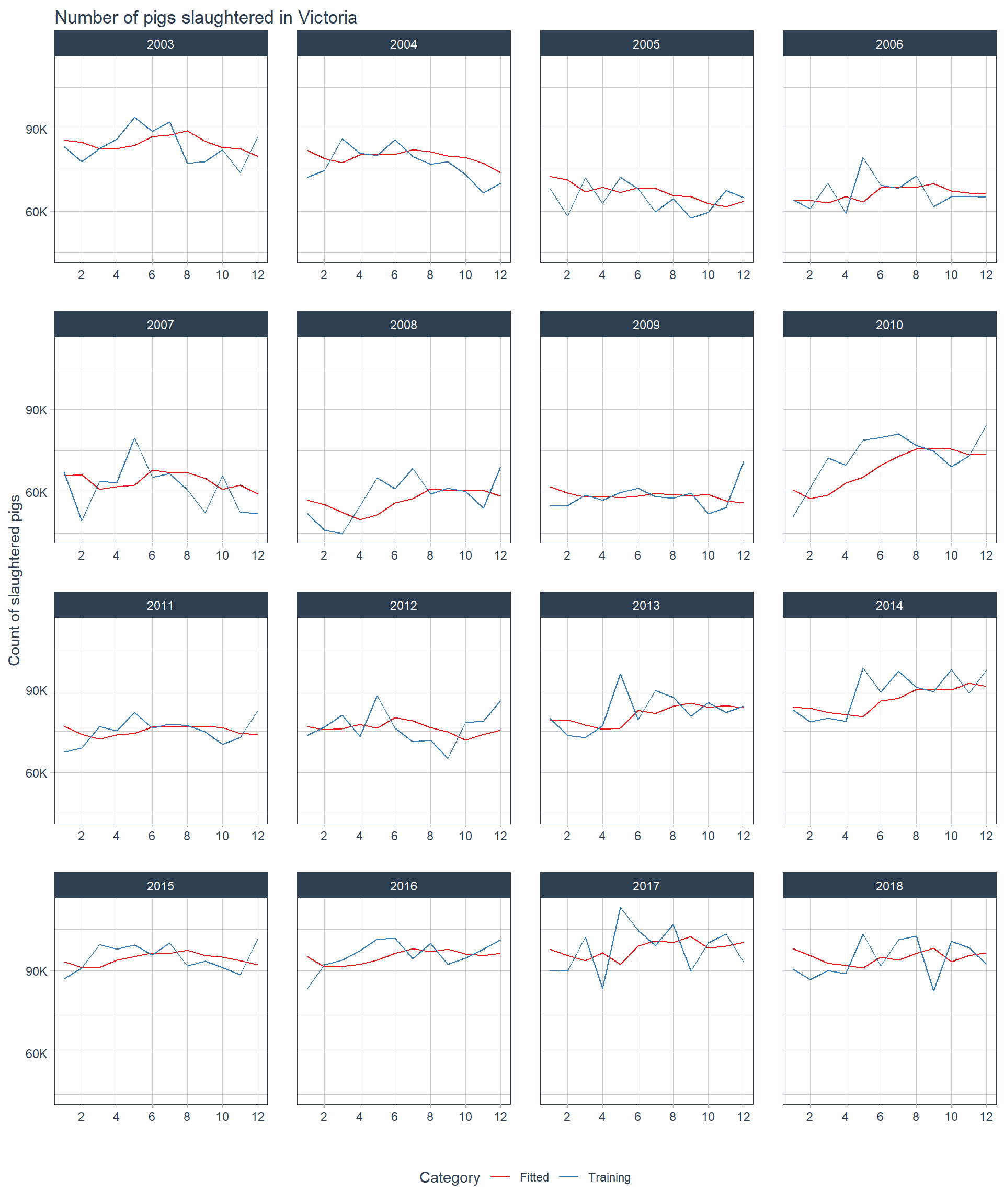
Do note that I wanted to see the performance for each year, but since the dataset is really long time-wise, I’ve decided to show period from 2003 onwards.↩︎
For more programmatically inclined readers, yes, this could have been done through recursion, but R was complaining.↩︎